See the limit of the mine, the yard, and the blending plant before you decide.
Simulate the loading and hauling cycle, plan road and rail logistics, and size blending plants. Compare scenarios before investing or closing the month’s plan.
Planning and Optimization in Mining: Bulk Logistics, Open-Pit Operations, and Blending Plants (Simulation, Digital Twins, and Optimization)
In mining, the expensive decision is often the one that looks simple: buy one more truck, raise the month’s volume, install one more silo. Each of these choices moves a system in which loaders, trucks, crushing, scales, tipplers, rail, and yards share the same flow. A calculation with average values does not show where the queue forms, which piece of equipment limits the whole, or how much the plan asks beyond what the operation can move.
Enacom represents the whole system in a model, with the real variability of the operation, and compares scenarios before the investment or the plan becomes a commitment. In open-pit mining, the model simulates the loading, hauling, and crushing cycle and shows the point where the additional fleet only creates queues. In road and rail logistics, it plans receiving, internal handling, and dispatch from the next day to the next month and measures the bottleneck by material. In blending plants, it sizes the number and capacity of silos from the inflow and outflow rates of each material.
We start from your operation: we represent the flow, calibrate the model with your data, and compare the alternatives before the decision.
3documented mining cases: open-pit mining, road and rail logistics, and silo blending
Up to 4%productivity gain in the simulated loading and hauling scenarios
−15%in silo installation costs and +20% operating efficiency, in the scenario comparison of a coal blending plant
D+1 to M+1horizon covered by the same road and rail logistics model
Why it works: the investment and the plan are tested against the whole system
In mining, each area’s result depends on the others: the mine depends on the crusher, the crusher on the fleet, logistics on the single track and the tipplers. When each decision is assessed in isolation, the limit only shows up in execution. The solution puts the whole cycle in the same model.
Invest where output responds
The simulation shows the point at which more trucks stop raising output and start forming queues. In an open-pit mine case, optimizing loading, hauling, and dumping times pointed to productivity gains of up to 4% in the simulated scenarios.
A plan that fits the logistics
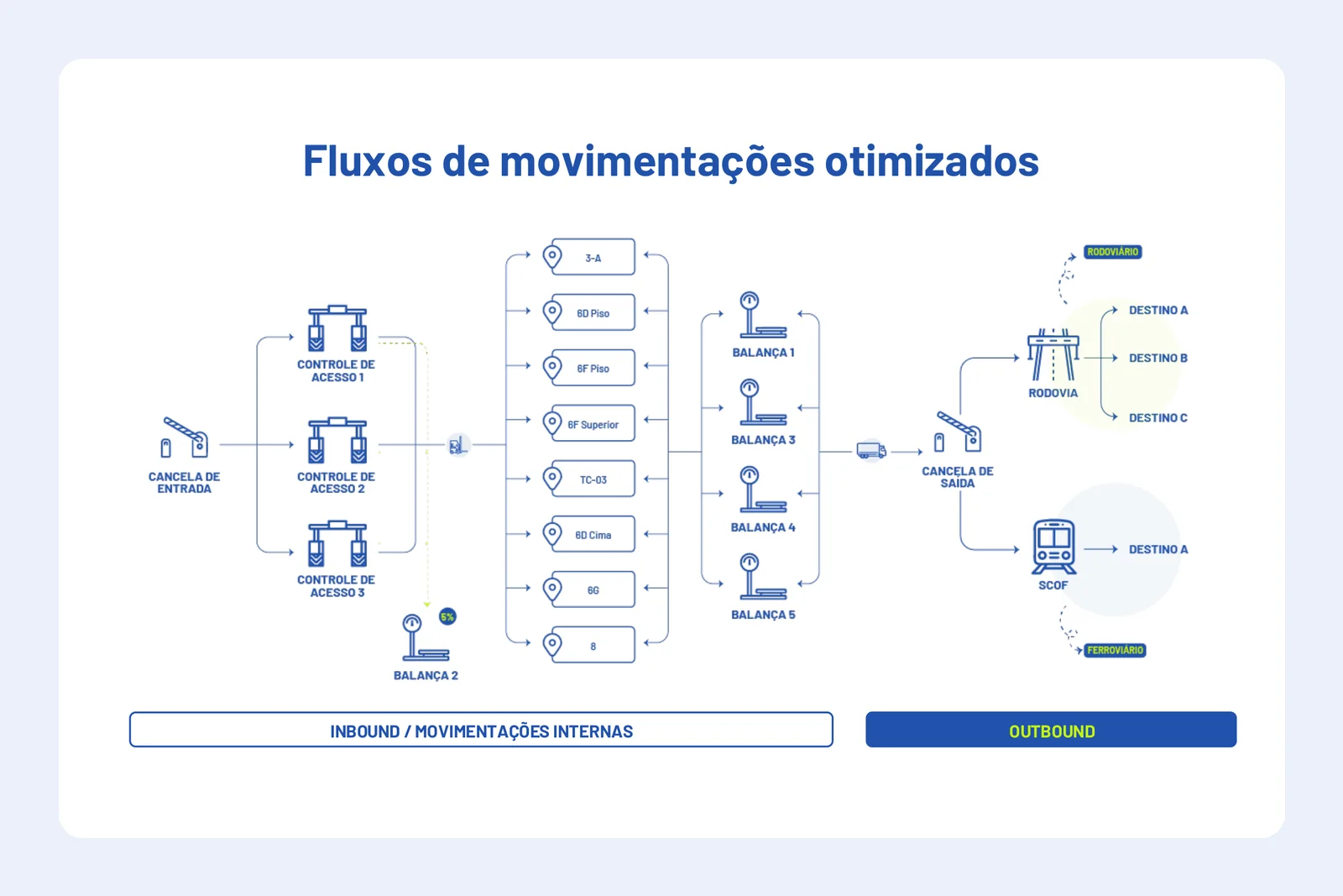
The desired volume of each material is checked against what gates, scales, yards, tipplers, and the exit track can move. The plan can grow where there is slack and be reduced where there is a bottleneck, with the limit in view before the month starts.
A plant sized by its flow
The number and capacity of the silos start from the inflow and outflow rates of each material. In a coal blending plant case, the optimized configuration indicated 15% lower installation cost and 20% higher operating efficiency in the scenario comparison.
Decision validated before scaling
We start from one specific decision, with your data, and compare scenarios before any purchase or plant change. The risk is small and the result is checked early.
Financial return. The value in reais depends on the scale and cost of each operation. We calculate the return and the payback period with your company’s data, before expanding the project.
Road and Rail Bulk Logistics: Receiving, Internal Handling, and Dispatch (D+1 to M+1 Planning)
The planned volume only materializes if the whole chain keeps up. The decision is how much of each material can actually pass through gates, scales, yards, tipplers, and the exit track, and where the bottleneck is.
Receiving and Effective Unloading Capacity (Inbound and Tipplers)
The model determines the effective capacity for receiving and unloading raw materials, with the demand for trucks and locomotives, the bottlenecks at the tipplers, the average cycle time per material, and the occupancy rate of the single track.
Internal Handling between Production Areas and Yards (Alternative Flows)
The optimizer calculates the maximum quantity of products processed and the number of locomotives and wagons required, and simulates alternative flows between production areas and yards to identify the ones that carry the greatest volume.
Road and Rail Dispatch (Outbound and Track Occupancy)
Dispatch by road and rail is modeled with vehicle demand, cycle time, and track occupancy, and the arrival time of trucks at the mine comes from the system’s capacity, not from a fixed schedule.
Desired vs. Achievable Volume by Material (Bottleneck Detection)
The plan for each material is compared with the volume the operation can achieve, and the analysis shows where the plan can grow and where it needs to be reduced. It also shows the combinations of tippler availability that fit within the hours of the month without bottlenecking the system, which puts maintenance and logistics in the same conversation.
Reference. The road and rail logistics optimizer case describes the analyses the model offers to logistics planning, from the next day to the next month. See the road and rail logistics case
Open-Pit Mining: Loading and Hauling Cycle, Fleet Sizing, and Investment Prioritization (Discrete-Event Simulation)
Drilling, loading, and hauling can account for up to 50% of the operating costs of an open-pit mine. The decision is where to invest, in trucks, loaders, or crushing, knowing how each choice changes the whole cycle.
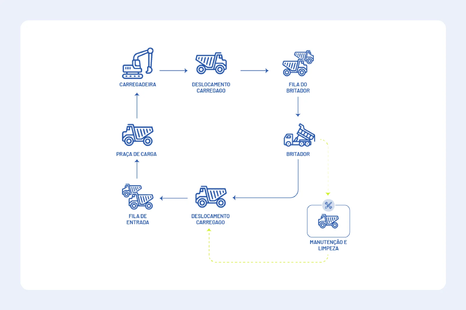
Loading, Hauling, and Crushing Cycle (Petri Nets)
The model represents the cycle from the loading area to the loader, the loaded haul, the queue and the crusher, and back to the entry queue, with detours for maintenance and cleaning. Petri nets are a technique for modeling discrete-event systems.
Fleet Saturation and Queue Formation (Fleet Sizing)
The simulation shows the point at which adding trucks stops increasing output: beyond it, the extra fleet creates queues at the loader and the crusher and lowers each truck’s productivity. The saturation point is visible before the purchase.
Real Load Variability (Probabilistic Simulation)
Each truck’s load varies from trip to trip. The model uses the distribution of the loads recorded on CAT-793C and CAT-793D trucks and simulates multiple trucks, queues, and parallel processes, instead of working with average values.
Investment Portfolio under a Budget Constraint (Capital Budgeting)
Trucks, loaders, and crushing compete for the same budget. Scenarios are compared by their effect on output, and the model builds the portfolio that delivers the most result within the budget limit. In the case, the model showed an error below 5% and was up to 3 times faster than other simulation methodologies.
Reference. The open-pit mine investment prioritization case presents the simulation results and the conditions under which they were obtained. See the open-pit mining case
Blending and Silo Sizing: Coal and Ore Blending Plants (Blend Optimization)
Too many silos make the installation more expensive, and too few run empty and interrupt the blend. The decision is how many silos to install, with what capacity, while keeping the proportion of each material.
Number and Capacity of Silos from Inflow and Outflow Rates
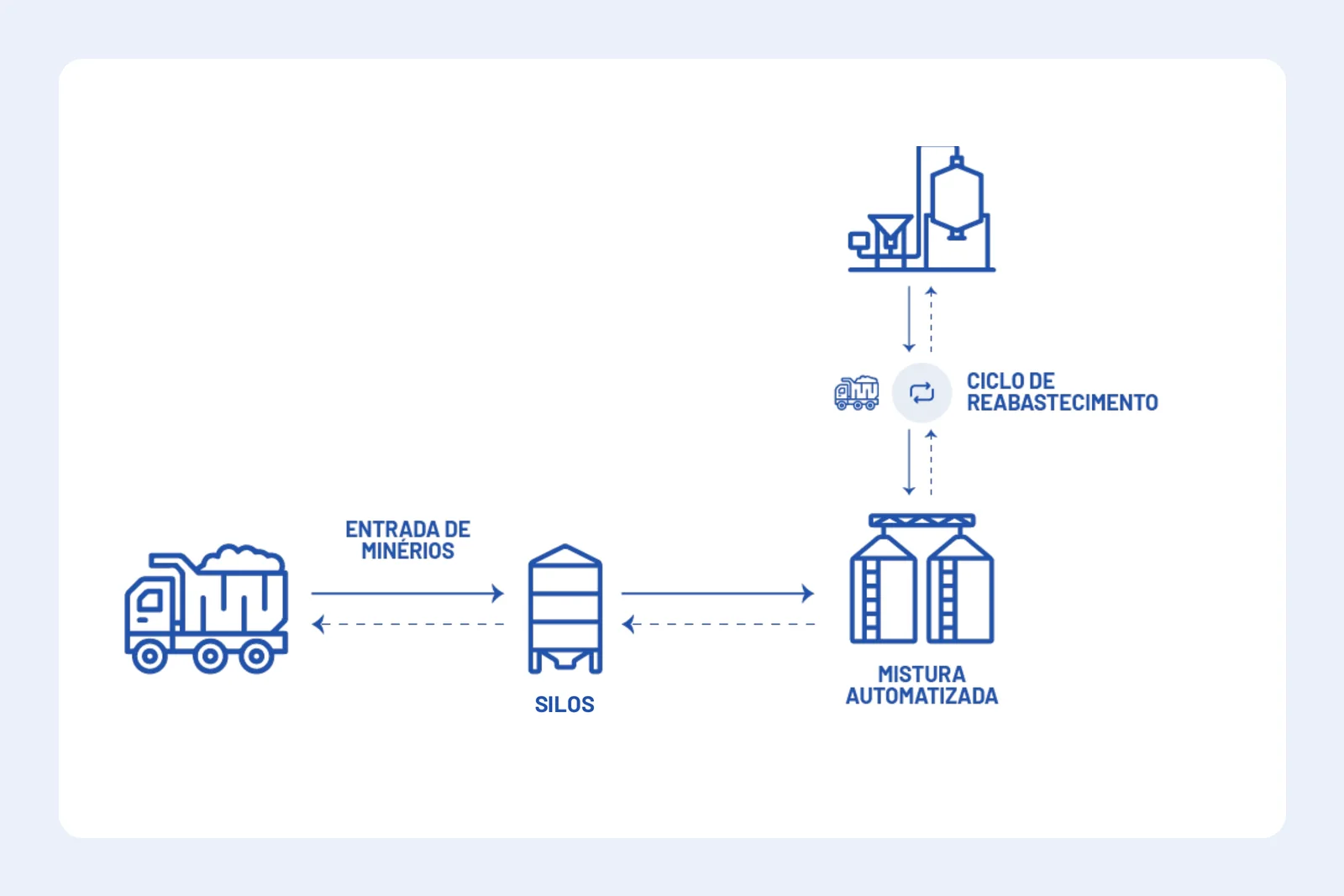
The analytical model calculates the number and capacity of the silos based on the inflow and outflow rates of each material, and compares scenarios until reaching the lowest-cost configuration that keeps the blend supplied.
Refilling Cycle in Sequence and Changeover Time
Refilling several silos has to be organized so that none runs empty and the changeover time is as short as possible. The optimization considers the refilling cycle in the sizing, not after it.
Proportion by Material and Stable Blend Quality
Each type of coal or ore has its own inflow rate and share. The model minimizes the total installation and operating cost of the silos while keeping the proportion of each material, which supports a stable-quality blend for production.
Quickly Implemented Heuristic Solution and Recipe Changes (What-if)
The heuristic speeds up the search without losing accuracy and allows adjusting the material types and their proportions in the blend, so new recipes can be tested in the model before changing the plant.
Reference. The blend optimizer and silo sizing case describes the scenario comparison that pointed to 15% lower installation cost and 20% higher operating efficiency. See the blending and silo case
Comparison: traditional approach vs. Enacom Digital Twin for mining
How each approach handles the criteria that define the quality of investment, logistics, and sizing decisions in mining.
Operating criterion
Spreadsheets and calculations with average values
Generic simulators and systems
Enacom Digital Twin (Gemminus Platform)
Loading and hauling cycle
Average productivity per truck, without queues
Simulation with standardized parameters
Full cycle in Petri nets, with queues, maintenance, and cleaning
Operating variability
Average load and time values
Generic distributions, poorly calibrated
Real distribution of the operation’s truck loads
Fleet size
Rule of thumb or history
Scenarios limited to fixed parameters
Saturation point visible before the purchase
Road and rail logistics
A plan per area, without the track and tippler capacity
Separate modules for each stage
Receiving, internal handling, and dispatch in the same model, from D+1 to M+1
Silo sizing
Sizing by design rule
Isolated calculation of each silo
Number and capacity from inflow and outflow rates, with the refilling cycle
Return focus
Keeping the routine
Tool standardization
Investment and plan compared by their effect on output and real capacity
Mining on the Gemminus Platform: Flow Models and Integration with Operational Systems
Enacom’s mining models reuse the Gemminus platform, the same one that supports the Planning Digital Twin in other industries. The model represents the operation’s flow, takes the data the team already has, and returns comparable scenarios for the decision.
The path is gradual: represent the flow, calibrate with the operation’s data, compare alternatives on one specific decision, and only then expand use, with the team in control.
One reference for the areas: mine, logistics, and blending plant assessed on the same model, with explicit assumptions.
Comparable scenarios: fleet, investment, flow, and silo alternatives measured against the same baseline.
Real variability: the operation is represented with the distribution of its own data, not with averages.
How to Start: Flow Mapping, a Model Calibrated with Your Data, and a Pilot on One Decision
In mining, the project starts from the operation’s flow and picks a decision where comparing scenarios makes a difference before the investment.
1. Mapping the flow and the constraints
We survey the mine cycle, the receiving, internal handling, and dispatch flows, or the rates and proportions of each blend material, together with the equipment and the constraints that limit each stage.
2. A model calibrated with the operation’s data
We build the model with real variability, such as the distribution of loads and the cycle times, and review the assumptions with the areas involved.
3. Pilot of one specific decision
We choose one decision, such as fleet size, the month’s volume plan, or the number of silos, and compare scenarios on the same reference before any purchase or change.
4. From the study to the planning routine
With the pilot validated, we define with the team how the model starts supporting short- and long-term planning, and which systems it connects to.
Frequently asked questions about planning and optimization in mining
What does Enacom do for mining?
It represents the operation’s system in a model, such as the loading and hauling cycle of an open-pit mine, the road and rail logistics of bulk materials, or a blending plant, and compares scenarios before investments and plans become commitments.
Why simulate instead of using average values?
Because each truck’s load and the times of each stage vary, and the queue only appears when that variation is considered. With average values, the point at which more trucks stop raising output is not visible.
Was the gain of up to 4% in productivity measured in the operation?
No. It is a simulation result, obtained in the scenarios evaluated, and the value is the maximum among them. The results of each case reflect the conditions of the operation analyzed.
Is the logistics optimizer only for mining?
It was developed for a bulk-materials operation that receives and ships by road and rail, with shared yards, scales, and tipplers, and the logic applies to other operations with those characteristics.
Where should we start?
With one specific decision, such as fleet size, the month’s volume, or silo sizing, with the flow mapped and the model calibrated with your operation’s data.
Go deeper into solutions, the platform, and Mining cases