
AISTech 2026, Pittsburgh, Pennsylvania (USA)
Heat Scheduling Optimization in Steelmaking
A heat scheduling algorithm for the steelmaking shop that minimizes free volume, demand delays, and co-scheduled steel grades, validated with real plant data.
Industrial application (Heat formation and steel shop scheduling)
Every heat in the steel shop has a fixed capacity, and orders rarely fill it. What is left becomes free volume: cast steel with no customer, sitting in the yard. The paper treats heat formation as a packing problem and makes explicit the order of what matters to the business.
From the mathematical concept to the business gain
- Knapsack Problem
- Fill each heat up to capacity with real orders, testing swaps between orders so that as little steel as possible is left without a destination.
- Lexicographic multi-objective optimization
- First reduce steel with no customer, then delivery delays, and only then resort to combining steel grades. A less important goal never worsens a more important one.
- Co-scheduling of steel grades
- Combine compatible grades in the same heat to complete its capacity, respecting the thickness, casting type and width of each strand.
Result: Over 12 months of real demand, combining grades cut free volume from 12.61% to 10.47% of the cast volume: 17% less steel with no customer in the yard, with an average early-demand volume of 1.37%.
See the case: Heat formationApplications in Steel
Enacom executive summary, based on the paper and the related projects.
Abstract
This study presents an optimization algorithm focused on heat scheduling in the steelmaking shop of a steel plant. The objective of the algorithm is to lexicographically minimize three critical aspects of the production process: free volume, demand delays, and the number of co-scheduled steel grades. The algorithm's performance was validated using real operational data from a steel plant, demonstrating its effectiveness in improving operational efficiency and reducing costs. The results indicate that, on average, 10.47% of the total casting volume corresponds to free volume when co-scheduling is considered, while early demand volume reaches an average of 1.37%.
Original abstract, published in English.
Keywords
Steel IndustryHeat FormationOptimizationKnapsack ProblemScheduling
View the publication on OnePetro
Full paper
Full text of the paper.
Introduction
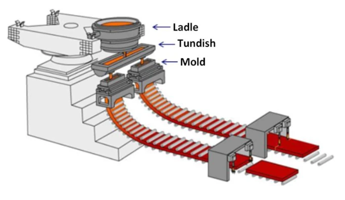
The manufacturing of steel products such as slabs, blooms, and billets involves several complex stages, ranging from the arrival of raw materials at the plant to the dispatch of finished products to customers. Proper management and optimization of these stages are essential to ensure efficient operation of the industrial plant and to achieve productivity gains.1 To this end, computer-assisted optimization tools combined with digital twin technologies can be employed.2, 3 These technologies have been applied across all stages of steel production, promoting productivity improvements and greater predictability throughout the production chain.4 Among the stages of steel production, continuous casting plays a crucial role in the production chain of a steel plant. After the hot metal undergoes refining processes in the steelmaking shop, the liquid steel is sent to the continuous casting stage, where it is transferred to the tundish. The tundish is responsible for feeding the molds in a controlled and continuous manner. During this process, the material begins to solidify and is shaped into semi-finished products such as slabs, blooms, or billets.5 Figure 1 presents a schematic representation of a continuous casting machine. The ladle pours the liquid steel into the tundish, which distributes the material among the molds. The molds, in turn, shape the steel into the desired geometry.6 After solidification and shaping, the products are cut and directed either to storage, sale, or further rolling processes.
Before initiating steel production, it is essential to determine which steel grades should be manufactured to meet specific customer demands. Each customer may request different steel compositions; therefore, the steel produced after continuous casting can vary according to order specifications. As a result, demands must be strategically grouped and organized so that customer due dates are met, and heats can be formed and cast sequentially. A heat corresponds to the volume of liquid steel generated from a single melting and refining operation, with a predefined chemical composition and metallurgical characteristics. Each heat has a maximum volume limit defined by the capacity of the steelmaking equipment.
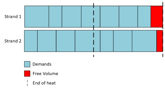
Within a group of heats that can be cast together, demands may present different volumes, and the sum of these volumes does not always exactly match the total capacity of the heat group. When excess steel is produced that is not associated with any specific demand, this excess is referred to as free volume. Figure 2 illustrates a group of heats composed of different demands and the corresponding free volume. In the figure, each blue rectangle represents a demand. The heats are separated by vertical dashed lines, and the free volume is indicated in red. The generation of this type of volume is undesirable, as it represents steel that is cast without a defined customer. After subsequent production stages, this steel tends to remain stored in yards without a clear destination, resulting in inventory accumulation and low logistical efficiency.
During the grouping of demands with similar steel characteristics for heat formation, it is possible to include steels with slightly different specifications through a process known as co-scheduling. In this context, co-schedulable steel is strategically produced within a heat originally intended for a steel grade with more stringent chemical composition and metallurgical requirements. This approach takes advantage of partial compatibility between steel grades, allowing the remaining heat volume—after fulfilling the primary demand—to be allocated to the production of a steel grade with fewer technical restrictions. As a result, process utilization is improved without compromising product quality.
This work aims to present an optimization algorithm capable of forming heats from a set of demands, with the goal of lexicographically minimizing the free volume generated, demand delays, and the number of co-scheduled steel grades. To this end, an algorithm based on the knapsack problem was developed and tested using real-world cases from a steel plant. This approach seeks to provide greater accuracy and agility in the heat formation process, since performing this task manually is time-consuming and requires significant operational effort.
Discussion
1. Problem Definition
This subsection presents a low-level definition of the heat formation problem for continuous casting in a steel plant. The definition describes the problem inputs and outputs, as well as the objective function and the associated constraints.
1.1 Inputs and Outputs
The main input parameters of the problem are:
- List of demands;
- List of heat groups;
- Thickness of the output product;
- Number of heats in the group;
- Number of strands;
- Strand widths;
- Steel grade;
- Product type;
- Casting type;
- Co-scheduling matrix;
- Steel charge consumed per heat;
- Yield of each casting type.
Each demand contains information regarding the steel grade, width, length, and thickness, product type, casting type, and due date. The list of heat groups stores information about sets of heats that will be cast together. Within each group, the output material thickness, the maximum number of heats, the number and width of strands, the steel grade, and the product type are defined. Each heat group specifies how the casting operations are configured.
The volume considered for each strand is given by the product of the number of heats and the steel charge consumed per heat. This volume is then used to allocate demands while respecting the imposed constraints. The co-scheduling matrix defines which steel grades are compatible with co-scheduling. The yield associated with each casting type determines the amount of steel lost during the casting process.
The output of the algorithm is a list of heat groups containing detailed information about the heats and the demands allocated to each strand.
1.2 Objective Function
The objective of the proposed algorithm is to lexicographically minimize the following factors:
- Free volume;
- Demand delays;
- Utilization of steel co-scheduling.
1.3 Hard Constraints
Hard constraints must be strictly satisfied all feasible solutions. The hard constraints of the problem are:
- The sum of demand volumes allocated to a heat group must not exceed the maximum capacity supported by that heat group;
- Heats within the same strand must contain demands with the same thickness and casting type;
- Demands allocated to heats must match the specified strand width;
- Each heat must be associated with at least one demand;
- The number of heats in each heat group is limited;
- Demands grouped within the same heat or heat group must be ordered according to their delivery due dates.
1.4 Soft Constraints
Soft constraints do not need to be strictly satisfied but are desirable to obtain solutions that are more aligned with operational and customer expectations. The soft constraints of the problem are:
- Heat groups should have the same steel grades, but they can have other grades, if co-schedulable, to improve heat yield;
- Demands should be balanced across strands, while prioritizing yield maximization;
- Pre-allocated demands should be selected first;
- The number of heats in each group represents a maximum value and may be reduced to avoid heats without allocated demands.
2. Main Algorithm
The aim of the optimization algorithm is to select, and group demands into a set of heats in order to lexicographically minimize free volume, demand delays, and the number of heats involving co-scheduled steel grades. Figure 3 presents the flowchart of the main algorithm.
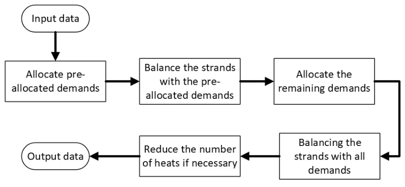
The first block addresses the allocation of pre-allocated demands. The second block performs the balancing of these demands across the strands, seeking to distribute similar demand volumes among them. The third block represents one of the core components of the algorithm, in which the remaining demands are allocated. The fourth block performs a rebalancing of all allocated demands. Finally, in the last block, empty heats are removed if no demands have been assigned to them.
The demand allocation procedure is based on a solution approach for the knapsack problem, in which the knapsack capacity corresponds to the sum of the volumes of the heats in each strand, and the item weights correspond to the demand volumes. The procedure consists of adding demands to the set of heats until the maximum capacity is reached, and no further demands can be accommodated. Subsequently, solution perturbations are applied in order to identify improved combinations of demands. At the end of the process, the best solution found is returned. This procedure is illustrated in Figure 4.
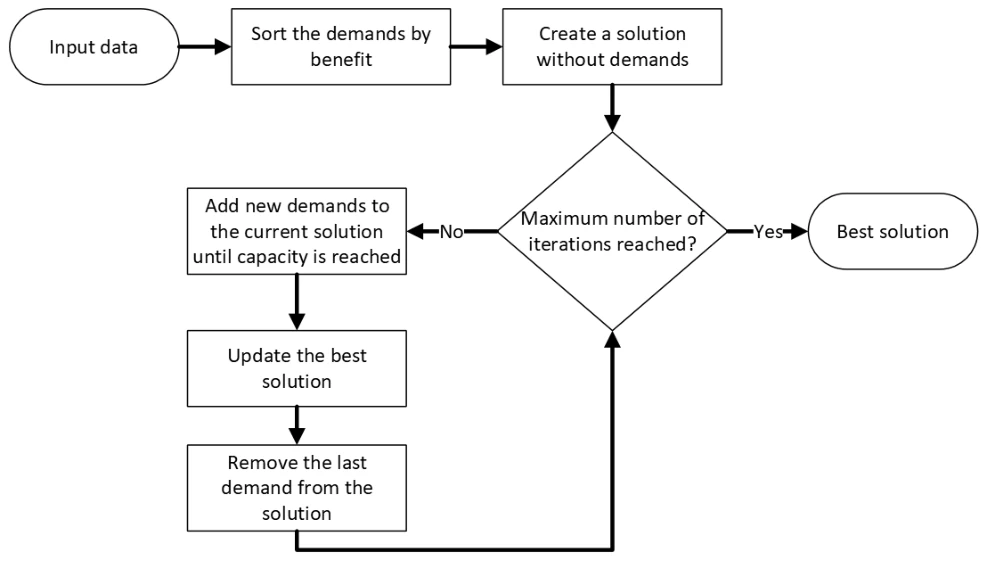
Initially, demands are sorted according to a priority score that takes into account demand volume, delivery delay, and whether the demand is co-schedulable. Next, an initial solution with no allocated demands is created. A solution can be interpreted as a set of knapsacks, where each knapsack corresponds to a heat group subdivided into strands. Subsequently, new demands are added to the current solution until the knapsack capacity is reached. The current best solution is then updated. Finally, the last demand added to the current solution is removed. This reduced solution is used in the next iteration in an attempt to construct alternative feasible solutions by adding different demands. The algorithm terminates when a predefined maximum number of iterations is reached. After completing all iterations, the best solution obtained is returned.
3. Results
The results were obtained by executing the algorithm on demand data covering a twelve-month period from a steel plant, in which heat formation was evaluated for two different rolling processes called ROLLING_1 and ROLLING_2. For each month, demands were grouped into scenarios corresponding to different reference dates, where each scenario contains a list of heat groups to which the demands must be allocated. These scenarios were analyzed under two different conditions: in the first, co-scheduling between different steel grades was allowed, while in the second, co-scheduling was not permitted. Of the scenarios analyzed, 77.44% are ROLLING_1 and 22.54% are ROLLING_2.
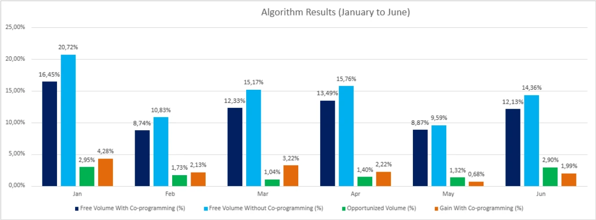
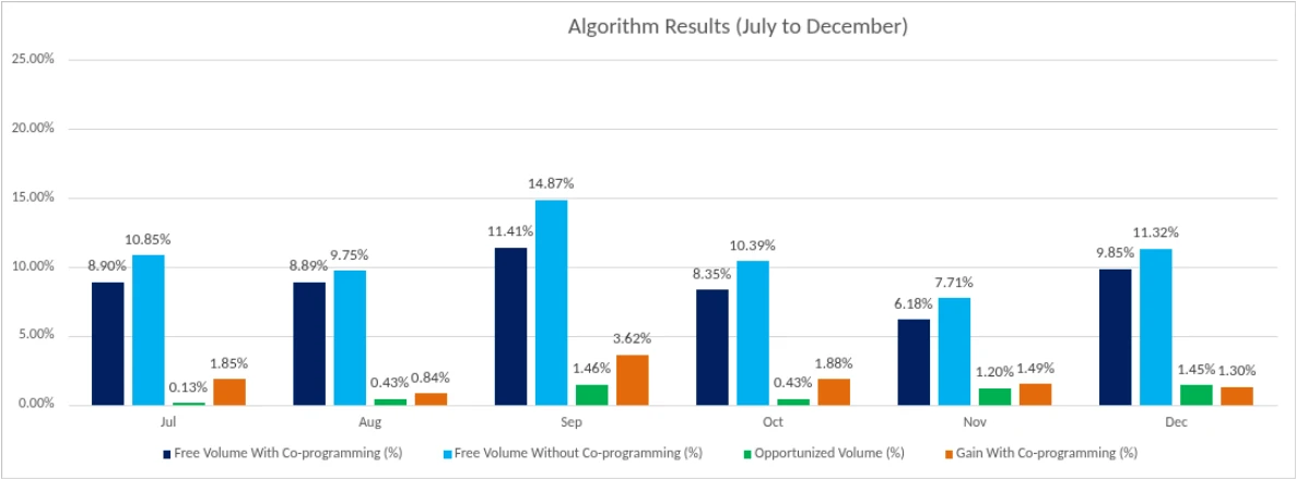
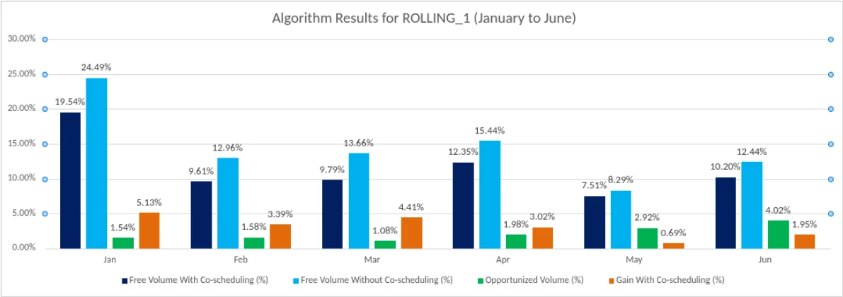
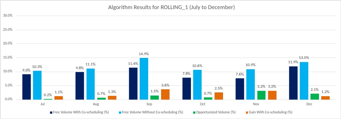
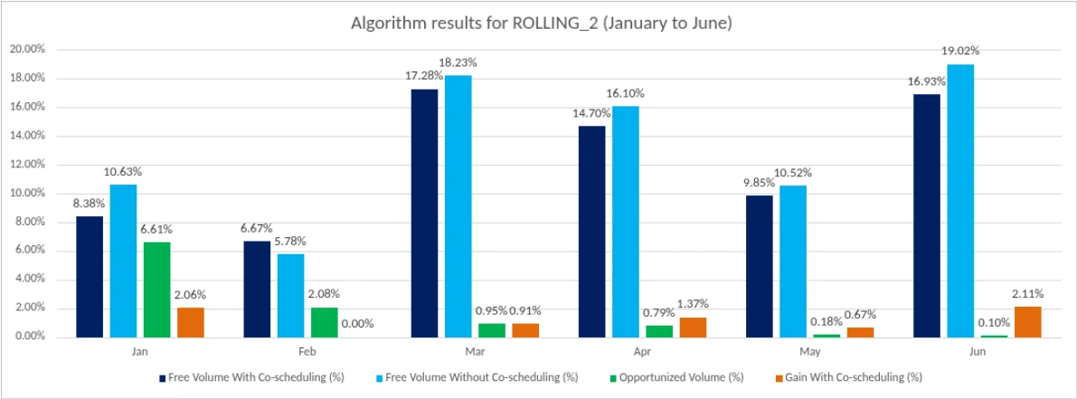
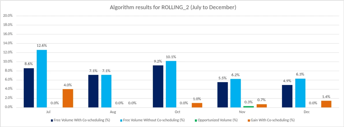
Figures 5 and 6 present a chart summarizing the main results of the algorithm for the scenarios described above. For each month, the figure shows the percentage of free volume with and without co-scheduling, as well as the percentage of opportunistic volumes and the gain obtained through co-scheduling. The early volume represents the demand volume that could be anticipated within a horizon of 10 days, while the co-scheduling gain corresponds to the volume of co-schedulable steel that was generated.
Table I supports the interpretation of the chart by presenting the average values of the evaluated parameters across the analyzed months. As can be observed, the free volume with co-scheduling over the four months was lower than the free volume obtained without considering co-scheduling. On average, the free volume with co-scheduling accounted for 10.47% of the total casting volume. In contrast, the scenario without co-scheduling resulted in an average free volume of 12.61%. This represents a reduction of 2.14 percentage points when comparing the scenarios with and without co-scheduling. This difference is mainly due to the possibility of completing heat groups using different, yet compatible, steel grades. On average, 1.37% of the total cast volume corresponds to co-schedulable demands that were anticipated within 14 days from the current date, while 2.12% of the total cast volume corresponds to co-schedulable steel.
| Parameter | Average |
|---|---|
| Free volume with co-scheduling | 10.47% |
| Free volume without co-scheduling | 12.61% |
| Advance volume | 1.37% |
| Gain from co-scheduling | 2.12% |
| Parameter | Average |
|---|---|
| Free volume with co-scheduling | 10.54% |
| Free volume without co-scheduling | 13.20% |
| Advance volume | 1.78% |
| Gain from co-scheduling | 2.62% |
For ROLLING_2, the results show lower free volume levels, both with and without co-scheduling. The early volume and the gains from co-scheduling are also lower than those observed in the aggregated case. This comparison highlights the importance of evaluating rolling processes individually, as their operational characteristics directly influence the benefits achievable through heat scheduling optimization.
| Parameter | Average |
|---|---|
| Free volume with co-scheduling | 9.91% |
| Free volume without co-scheduling | 11.14% |
| Advance volume | 1.00% |
| Gain from co-scheduling | 1.21% |
Conclusions
This work presented an optimization approach focused on heat formation for the continuous casting process in a steel plant, simultaneously considering the lexicographic minimization of three critical factors: the free volume generated, delivery delays, and the number of co-schedulable steel grades. The problem was modeled as a variant of the knapsack problem, in which demands correspond to items and a set of heats corresponds to the knapsack. The algorithm was tested using real operational data from a steel plant.
In addition to its practical potential, the proposed methodology offers flexibility for future adaptations, such as the inclusion of new constraints and the consideration of other steelmaking structures. As future work, the extension of heat formation to different products and plants is suggested, as well as integration with other digital twin systems already in operation within the same plant, such as the steelmaking and rolling mill digital twins. In these cases, the algorithm may both receive additional information from these digital twins and provide relevant information to support their operation and decision-making processes.
References
- J. Schulz, “Applying Mathematical Optimization in Practice,” SN Operations Research Forum, Vol. 2, No. 3, 2021, pp. 1–12, https://doi.org/10.1007/s43069-020-00046-9.
- Z.J. Xu, Z. Zheng and X.Q. Gao, “Operation Optimization of the Steel Manufacturing Process: A Brief Review,” International Journal of Minerals, Metallurgy and Materials, Vol. 28, No. 8, 2021, pp. 1274–1287, https://doi.org/10.1007/s12613-021-2273-7.
- M. Javaid, A. Haleem and R. Suman, “Digital Twin Applications Toward Industry 4.0: A Review,” Cognitive Robotics, Vol. 3, 2023, pp. 71–92, https://doi.org/10.1016/j.cogrob.2023.04.003
- Y. Zhang, M. Sukhram, I. Cameron and A. Rozo, “Industrial Perspective of Digital Twin Development and Applications for Iron and Steel Processes,” in AISTech 2020 Conference Proceedings, Association for Iron & Steel Technology, Warrendale, Pa., USA, 2021, pp. 34–43.
- J.K. Brimacombe, “Continuous Casting: The Saga of a Success Story,” Metallurgical and Materials Transactions B, Vol. 26, No. 5, 1995, pp. 761–785, https://doi.org/10.1007/BF02658134.
- I.R.S. Lana and T.F. Oliveira, “Influence of Argon Diffuser on Steel Cleanliness During the Continuous Casting Process,” in Proceedings of the 15th Enemet, Rio de Janeiro, Brazil, 2015, pp. 2713–2722, https://doi.org/10.5151/1516-392X- 26481.
Want to talk about what you read?
Tell us the challenge in your operation and our team will assess with you where to start.