
AISTech 2025, Nashville, Tennessee (USA)
Redefining Industrial Performance in the Era of Digital Twins
Three steel plant case studies show the limits of metrics such as OEE and propose Digital Twin approaches that measure performance from the production flow perspective.
Industrial application (Measuring industrial performance beyond OEE)
Conventional indicators such as OEE look at each piece of equipment in isolation. The paper shows what they miss in a steel mill and how to measure performance along the production flow.
From the mathematical concept to the business gain
- OEE limitations
- Losses that come from product mix, production routes or over-quality do not show up when each piece of equipment is measured alone.
- Flow-based performance
- The Digital Twin measures performance along the flow and links each loss to its cause in the value chain.
- Three case studies
- Effect of product mix, effect of routes on process times and incidence of over-quality, measured in a real mill.
Result: A more accurate, holistic view of operations that guides where to focus improvement efforts.
Performance Digital TwinApplications in Steel
Enacom executive summary, based on the paper and the related projects.
Abstract
Staying competitive in the industry is a major challenge. Given that a significant portion of this competitiveness stems from maximizing industrial performance, it is natural that the evolution of production monitoring tools plays a pivotal role in this process. Therefore, this article presents three case studies from a steel plant, addressing the imperative of optimizing operational efficiency in complex and interconnected processes. The first case study delves into the impact of product mix on manufacturing, considering various production scenarios. The second examines the influence of production routes on process times. The third one investigates the prevalence and characteristics of over-quality instances within the production process. The limitations of conventional performance metrics, such as OEE, are described and emphasized. Alternative approaches that employ Digital Twins to measure the performance from the production flow perspective are proposed. These approaches offer a holistic and more precise view of the operations and the value chain.
Original abstract, published in English.
View the publication on OnePetro
Full paper
Full text of the paper. Version presented at ABM Week 2024 (26th Automation and IT Seminar, São Paulo, Brazil, September 3–5, 2024); it may differ from the version published in the AISTech 2025 proceedings.
1 Introduction
In an increasingly dynamic and competitive environment, the pursuit of operational efficiency optimization is essential for the success of any organization [1]. In this journey, metrics play a crucial role by providing valuable insights to managers [2]. One such widely recognized and utilized metric is Overall Equipment Effectiveness (OEE), which focuses on measuring the productivity of industrial equipment, considering availability, performance, and quality [3].
However, despite being functional for their initial purposes and widely disseminated, asset-focused metrics and isolated analyses, such as OEE, have limitations when the goal is to increase the efficiency of the entire production process, especially when it involves interrelated equipment [4].
The current scenario, enveloped in the Industry 4.0 revolution, increasingly demands an integrated and comprehensive approach, particularly with complex industrial operations [5]. Often, these processes involve equipment interdependence, production of multiple SKUs (Stock Keeping Unit), and product-sensitive processes, requiring holistic measurements and performance analyses, integrating the entire production flow.
The focal point is that manufacturing processes become increasingly intelligent and digitized [6]. In response to this necessity, as a product of Industry 4.0, the concept of Digital Twin emerges [7], offering a more holistic and precise view of industrial operations and the value chain. A Digital Twin can be considered an idea referring to a virtual representation of manufacturing elements, such as personnel, products, assets, and process definitions, a living model that updates and changes continuously as the corresponding physical counterpart changes to represent statuses, working conditions, product geometries, and resource states [8].
This article presents two case studies for steelmaking manufacturing processes, aiming to highlight the need for utilizing a Digital Twin in production process analysis and the limitations of metrics focused on isolated processes.
2 Development
For effective production planning, it is necessary to have a better understanding of each stage of the process and how they relate to each other, as well as how the performance of each asset can be influenced by the item being produced. To demonstrate this, two case studies are presented. The Digital Twin of Performance from Enacom is used as a basis for the methodologies employed in solving the presented problems.
2.1 Impact of SKU production mix on production targets
For this analysis, a scenario is considered in which the production capacity for the next month of an industrial steelmaking process of a company is estimated, focusing on two isolated SKUs, based on the company's historical data. The goal is to obtain an initial estimate of the range of items produced that will be achieved in the following month, in order to assist in choosing the portfolio composition.
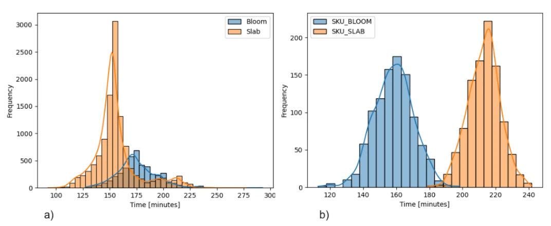
The data used ranged from January to December 2023. Figure 1a shows the historical distributions of the process. For a more detailed perspective, one SKU from the bloom casting and one from the slab casting were used. Statistical parameters for the distribution of lead-times (total production time of the item) for each SKU over the entire period were obtained, and using the normal distribution, with 1000 values for each of the SKUs analyzed, the samplings were made and are presented in Figure 1b.
| SKU | Mean [min] | Std* [min] | Category mean** [min] | Category std* [min] |
|---|---|---|---|---|
| SKU_BLOOM | 158.40 | 11.96 | 178.75 | 18.60 |
| SKU_SLAB | 212.88 | 9.63 | 162.84 | 20.63 |
| Mean | 185.64 | 29.32 | 160.45 | 21.97 |
* Standard deviation.
** The values for the entire category are considered for the analyzed period, regardless of SKU.
In a simplistic analysis, based on the historical process average (160.45 min), the estimated quantity of items produced for the next month could be calculated using Equation 1, given the 43,200 available minutes (assuming 30 uninterrupted working days).

where T is available time and tp is the average time of process.
This would result in a value of 269 items produced in the next month. However, as illustrated in Figure 1b, the data exhibits a multimodal distribution, indicating that a single average is not able to represent all the data. This becomes evident in Table 1 when comparing the averages between the two SKUs, where the average time required to produce SKU_BLOOM is approximately 55 minutes less than for SKU_SLAB.
Furthermore, upon further analysis of Table 1, it is apparent that a slightly less simplistic but still generic approach, which would be to consider the average times of each contingent as their respective references, would also not be adequate. This is because, although historically the production of SKUs from the casting slab is slightly faster than that of the casting bloom (Figure 1a), for the chosen products, the situation is reversed.
Therefore, it can be concluded that the lead-time distribution varies according to the SKU, and the use of generalizations is not suitable. It is inferred that the production estimation methodology should consider more specific data of what is intended to be executed with the desired combinations.
Moreover, even considering that only one item can be produced at a time, in full, which would allow the use of Equation 1, but being segregated by SKU, and with detailed process times available, two questions emerge: (i) How much available time should be considered for each SKU? (ii) What level of risk in the estimation can be accepted?
These are questions that require a higher level of detail about the process, both from historical data and from adaptation to what is intended to be simulated, intrinsic characteristics of a Digital Twin. The first question is associated with the scheduler's expectation of the production mix. This means that, as items compete for resources (time, in this case), the priority of use for each SKU must be established. The second question is associated with how process dispersion can influence results.
Through the methodology of Enacom's Performance Digital Twin, the probability curves of portfolio production as a function of process dispersion were obtained, as shown in Figure 2. Five curves are presented: three reflecting the impact of portfolio composition, varying the percentage of time assigned to each SKU in the process; and two presenting reference values, one with the calculation made considering the average times between the two analyzed SKUs and the other considering the average time of the process.
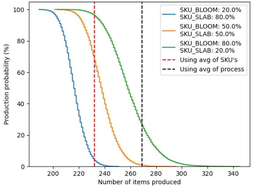
The result depicted in Figure 2 is a probability curve where each point represents how likely it is to produce a certain quantity of items, given a portfolio. It highlights that the predicted quantity of items produced is not absolute, but rather dependent on the risk one wishes to assume (considering how unlikely it is to achieve such a result) and the proportions used in the product mix. It also shows that the fulfillment curve shifts depending on the demand mix, exhibiting larger production behaviors with increased demand for SKU_BLOOM. Such behavior could be expected, as it has lower times than SKU_SLAB, as seen in Table 1.
It is worth noting that each planning scenario (mix used and risk assumed) is a point on one of these curves. Note that if only some average values were assumed for the estimate (dashed vertical lines), the result would be an absolute value that could be considerably far from the probable, depending on the mix used, as shown in Table 2.
| Combination (SKU A–SKU B)* | Probable number of items (50%) | Probability of estimated method occurrence: avg of SKUs’ times (233 items) | Probability of estimated method occurrence: avg of process’ times (269 items) |
|---|---|---|---|
| 20-80 | 216 | 3.99% | 0.00% |
| 50-50 | 238 | 67.37% | 0.86% |
| 80-20 | 258 | 96.10% | 26.16% |
*SKU A: SKU_BLOOM and SKU B: SKU_SLAB
80-20 258 96.10% 26.16%
Note that if the estimate of items produced in the month were made without considering the product mix, it would return probable values of 233 items for the method considering the average of SKU times and 269 items considering the average of process times. However, the probability of 233 items being produced does not reach 4% for the first configuration; it is close to the most probable estimate for the second configuration, which is 238 items, and reaches 96% probability for the third case. Furthermore, if the average of process times is considered, which would mean focusing only on the asset instead of a holistic view, the best chances would be for the third combination, but still not reaching 30% probability. It would be practically impossible to achieve such a quantity for the other configurations.
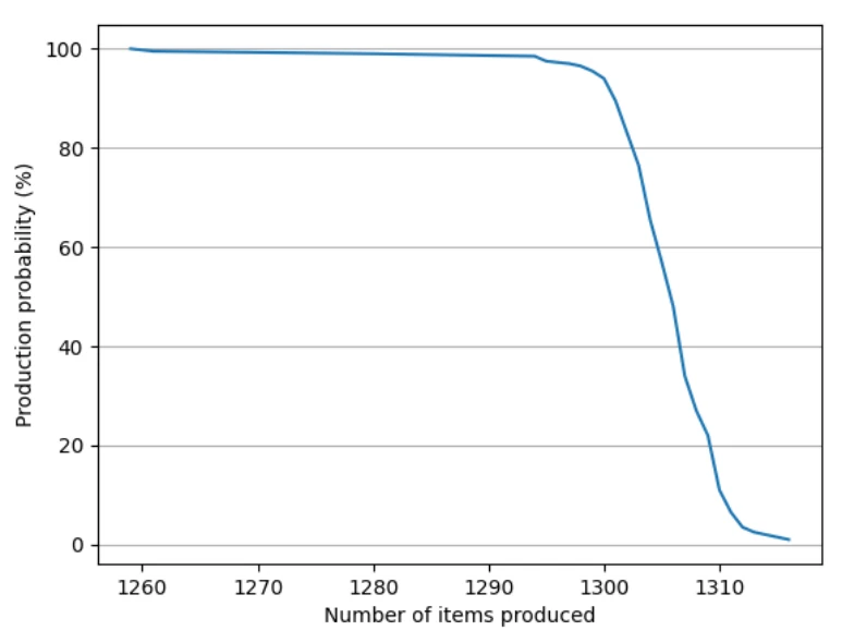
As mentioned earlier, this case presents abstractions in the way of estimating production for the subsequent month. Like in a Digital Twin, it should still be considered that, to produce an SKU, more than one process is executed, with or without competition, depending on the product category, and the possibility of parallel processes, such as machines that perform the same function. Incorporating such details into the analysis, the number of items obtained would show a significant disparity with the simple metrics used, corroborating the idea of the inefficiency of using asset-focused methods instead of holistic methods. Figure 3 presents the result obtained by Enacom's Performance Digital Twin for the case of a 50% mix for each of the SKUs.
2.1 Impact of production route on process times definition and decision making
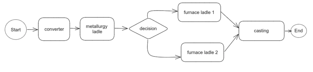
For this analysis, a scenario is considered in which a single SKU, from casting slab type, is produced, and there is a decision to take two distinct routes, which differ by the choice between two equivalent equipment. A schematic is depicted in Figure 4.
Assuming equal production costs on each machine and the goal of maximizing production, the allocation decision is to define the allocation proportion in each production route, aiming to minimize the total process time. Figure 5 presents the statistical distribution of process times in the ladle furnaces. The data in this section are based on samplings of 1000 values from the historical distribution of processes.
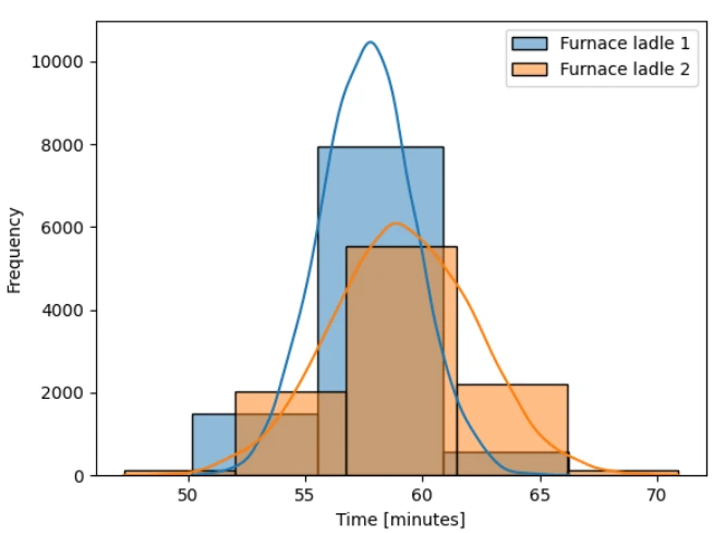
The average production times on the machines are 57.67 minutes for Ladle Furnace 1 and 59.22 minutes for Ladle Furnace 2. Consequently, the immediate natural conclusion is that Ladle Furnace 1 should be prioritized over Ladle Furnace 2 in order to produce the highest possible number of items. However, this conclusion should not be obtained in such a simplified manner because it would only be true if the processing time on each machine presented in the schematic of Figure 4 were independent of the overall path. However, as can be observed in Figure 6, the processing time in ladle metallurgy is historically influenced by the ladle furnace used previously.
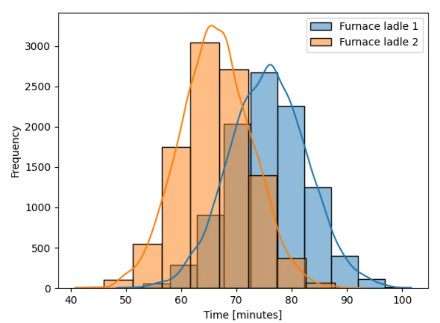
The average production time in ladle metallurgy is 70.93 minutes. However, the average time when the previous process was carried out in Furnace Ladle 1 is 75.64 minutes compared to 66.21 minutes when Furnace Ladle 2 was used. Note how holistic flow-oriented analysis, rather than isolated process analysis, can influence decision-making, as it can change the perception of which route is most productive. Table 3 presents a comparison between the times, disregarding the process times in the Converter and in Metallurgy Ladle.
| Route | Sum of process times [min]: analysis by assets | Sum of process times [min]: analysis by route |
|---|---|---|
| Furnace Ladle 1 -> Casting | 128.60 | 133.28 |
| Furnace Ladle 2 -> Casting | 130.15 | 125.42 |
A variation of approximately 2.5% in time is observed simply by guiding resource allocation decisions with more refined data, considering correlations between them, rather than a simplistic analysis based on averages of asset performances in isolation.
3 Conclusion
Redefining industrial performance in the era of Digital Twins is essential for competitiveness and success in modern industrial operations. Through simplified examples representing complex industrial processes, the importance of striving for operational efficiency optimization by embracing a more holistic and integrated approach has been demonstrated, overcoming the limitations of traditional metrics, which are focused on isolated analyses and asset-centric approaches.
The integration of the Digital Twin concept emerges as a promising solution for detailed performance analysis, considering complex variables such as SKU production mix and production routes. By disaggregating performance data by SKU and simulating different production scenarios, it is possible to obtain a more precise view of production capacity and make more informed decisions.
Acknowledgments
This work was supported by CAPES, CNPq and FAPEMIG, Brazil.
References
- Oliveira R, Taki SA, Sousa S, Salimi MA. Global Process Effectiveness: When Overall Equipment Effectiveness Meets Adherence to Schedule. Procedia Manufacturing. 2009; 38, 1615–1622. https://doi.org/10.1016/J.PROMFG.2020.01.123.
- Jasiulewicz-Kaczmarek M, Piechowski M, Szafer P. Practical Aspects of OEE in Automotive Company - Case Study. Proceedings of International Conference on Management Science and Management Innovation August. 2016; 13- 14.https://doi.org/10.2991/msmi-16.2016.51.
- Muchiri P, Pintelon L. Performance measurement using overall equipment effectiveness (OEE): Literature review and practical application discussion. International Journal of Production Research. 2008; 46 (13), 3517–3535. https://doi.org/10.1080/00207540601142645.
- Braglia M, Frosolini M, Zammori F. Overall Equipment effectiveness of a manufacturing line (OEEML) - an integrated approach to assess systems performance. Journal of Manufacturing Technology Management. 2009; v.20, n.1, pp. 8-29.
- Boyes H, Hallaq B, Cunningham J, Watson T. The industrial internet of things (IIoT): an analysis framework. Comput. Industry 101. 2018; 1–12, https://doi.org/10.1016/j.compind.2018.04.015.
- Nazarenko AA, Sarraipa J, Camarinha-Matos LM, Grunewald C, Dorchain M, Jardim-Goncalves R. Analysis of relevant standards for industrial systems to support zero defects manufacturing process. Journal of Industrial Information Integration. 2021; 23, 100214. https://doi.org/10.1016/J.JII.2021.100214.
- Foidl H, Felderer M. Research challenges of industry 4.0 for quality management. Lecture Notes in Business Information Processing, 2016; 245, 121-137. https://doi.org/ 10.1007/978-3-319-32799-0_10.
- Lu Y, Liu C, Wang KIK, Huang H, Xu X. Digital Twin-driven smart manufacturing: Connotation, reference model, applications and research issues. Robotics and Computer-Integrated Manufacturing. 2020; 61, 101837. https://doi.org/10.1016/J.RCIM.2019.101837
Want to talk about what you read?
Tell us the challenge in your operation and our team will assess with you where to start.